3) Multiple Linear Regression

 Multiple Linear Regression

Here we have multiple features such as (x1,x2,x3...) instead of one feature (x1) and after feed these features to model we can get the output (y). Before proceeding away we should understand some of the terminologies which we use for ML. let's assume a[i][j] here will the help of j we can proceed toward columns and with the help of i we can proceed toward rows. Furthermore, n is the total number features.

How Model find value for Multiple Features:

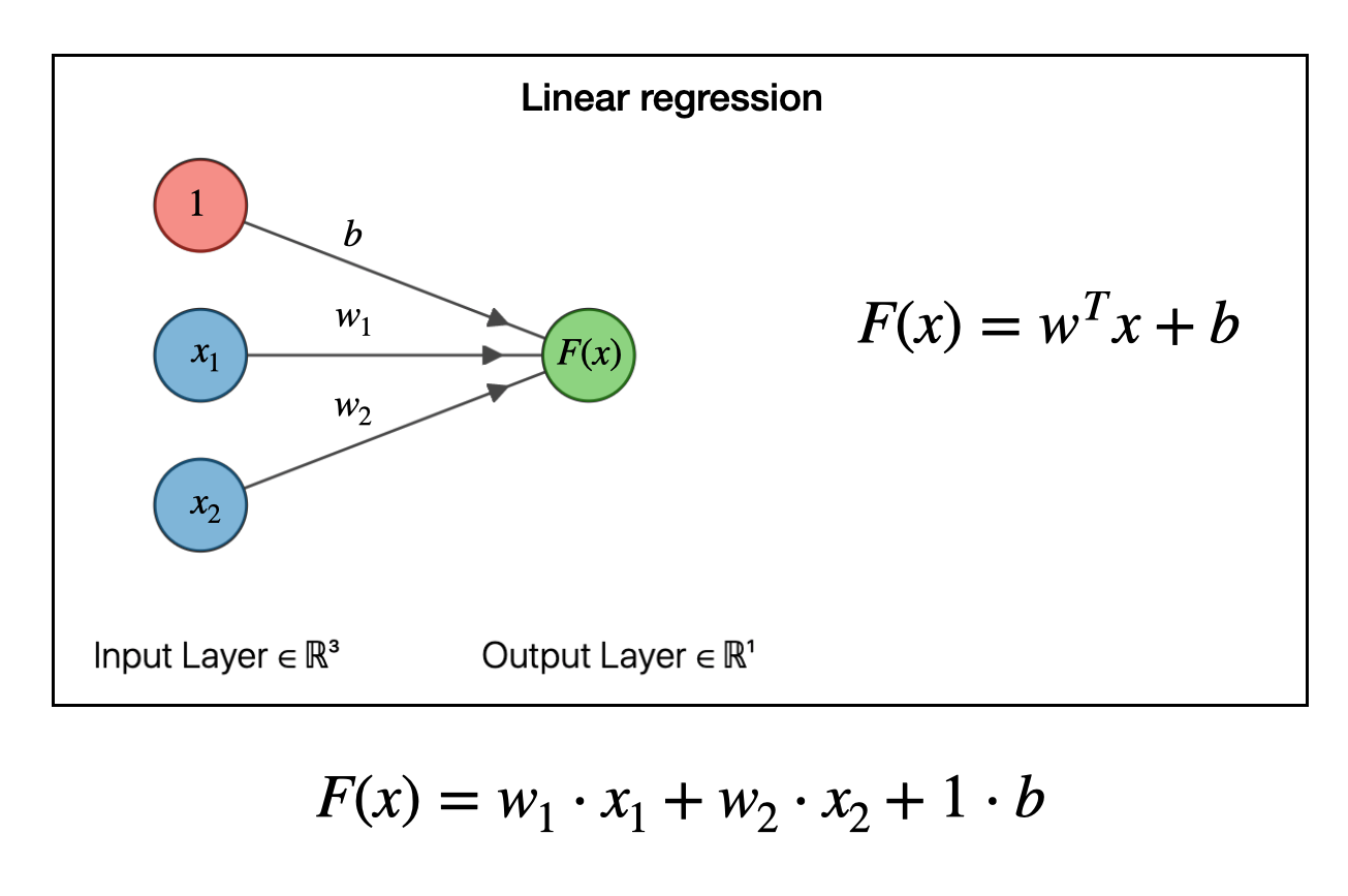
let’s assume we have 3 features x1, x2 and x3 with three weights w1, w2, w3 and one bias b and by using these values we can find the output f(x).

f(x)= ((x1*w1)+(x2*w2)+(x3*w3))+b

After getting the f(x) value we go ahead by finding the loss with the help of loss function and apply gradient decent to get the right parameters (weight and bias) for the model. This all we will understand with time. But for now we should have little bit of understanding for basic terminologies, methods and approaches.

=> We have bias b, weights [w1,w2,w3..] and features [x1,x2,x3…]

=> Model f(x)= pred_y[ i ] =w1*x1+w2*x2+…+w(n)*x(n)

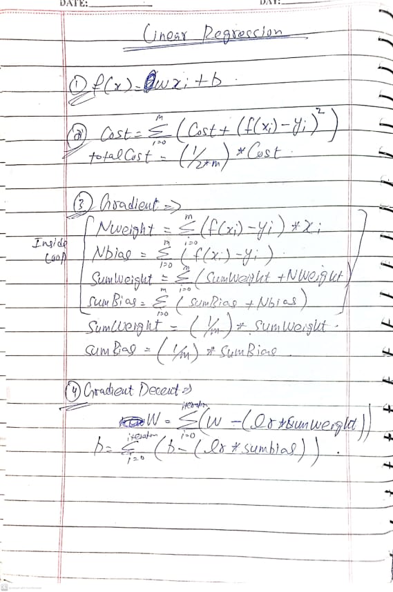
=> cost function J(w[i],b)=((sigma(pred_y[i]- actual_y[i]))²)/2m

=>update weight w[i]= w[i]- learning rate * ( J(w[i], b ) * x[i]

=>update bias b= b- learning rate * (J(w[i],b)

Note: Vectorization is good approach to perform any operation as compare to use loops

Here we have Model named as f(x) and with the help of model we predict our output (y). After predicting the value (y) we will find the error using cost function called Gradient decent. Our parameters will perfectly tuned if our cost function is close to zero. With the help of cost function we will find the cost between actual_y (output) and predicted_y (output). If our error is high then we will update the weight and bias and make the cost close to 0.

Feature Scaling:

In simple word this is normalization of independent features. This helps us make gradient fast. We use normalization if either feature difference is too small or too large. Therefore, in normalization we scale the values between 0 and 1 most of the case. We can take the example of images while training model for images we normalize the images to make training fast for model. There are too much types of normalization and mostly common two of them are given below

1) Z-Score Normalization: Here data (features) will normalize in such that mean of your data will be zero and standard derivation will become 1.

               Formula:          x1= ( x1 - mean( u1 ) ) / ( standard deviation )

2) Mean Normalization:   Here we normalize the data with respect to mean

             

               Formula:           x1= ( x1 - mean( u1 ) ) / ( max - min )

Note: Now a days features engineering is one of the most useful thing in ML because with the help of it we identifies news features for model

An overview Diagram of Linear Regression:

Notes for Linear Regression:

I made very simplified version linear regression Code (Python) which is given below:

import numpy as np
import matplotlib.pyplot as plt
xFeatures=np.array([2,3])
yFeatures=np.array([330,400])
# plt.scatter(xFeatures,yFeatures,marker='x',c='r')
# plt.title("Actual Values")
# plt.xlabel("Size")
# plt.ylabel("Price")
# plt.show()
lr=0.1
m=len(xFeatures)
def calculate(x,w,b):
    y=w*x+b
    return y
def cost(x,y,w,b):
    JSumWeight=0
    m=len(x)
    for i in range(m):
        f_wb=(w*x[i])+b
        JSumWeight=JSumWeight+np.power((f_wb-y[i]),2)
    totalCostW=(1/2*m)*JSumWeight
    return totalCostW

def gDecent(x,y,w,b):
    wid=0
    bs=0
    sumWeights=0
    sumBias=0
    for i in range(len(x)):
        f_wb=(w*x[i])+b
        wid=(f_wb-y[i])*x[i]
        bs=(f_wb-y[i])
        sumWeights+=wid
        sumBias+=bs
        
    sumWeights=(1/m)*(sumWeights)
    sumBias=(1/m)*(sumBias)
    return sumWeights,sumBias
            
def resultGDecent(x,y,w,b,iterations):
    recordW=np.zeros(iterations)
    recordB=np.zeros(iterations)
    for i in range(iterations):
        errorW,errorB=gDecent(x,y,w,b)
        newW=w-(lr*errorW)
        newB=b-(lr*errorB)
        w=newW
        b=newB
        recordW[i]=w
        recordB[i]=b
    
    return recordW,recordB

bias=1
weight=0.25
w,b=resultGDecent(xFeatures,yFeatures,weight,bias,1000)
print("1st Weight is ",w)
print("1st Bias is ",b)

# w,b=resultGDecent(xFeatures,yFeatures,w,b)
# print("Last Weight is ",w)
# print("Last Bias is ",b)
# w,b=resultGDecent(xFeatures,yFeatures,w,b)
# print("Last 1 Weight is ",w)
# print("Last 1 Bias is ",b)
getCost=cost(xFeatures,yFeatures,w,b)
print("Cost is ",getCost)
# plt.scatter(w,b,marker='x',c='r')
# plt.title("Actual Values")
# plt.xlabel("Width")
# plt.ylabel("Height")
# plt.show()
print("Our real value is ",xFeatures*w[-1]+b[-1])

Output:
After updating weights and bias we will have predicted value below
Our predicted value (y) is [328.882757 400.78734259]
You can check the actual y above in the code. For features x our model is predicting these values y after updating weights and bias with the help of gradient decent.
For Now this is enough. Today we learn some of the terminologies and functions which helps us for training model and updating weights and bias. We also see the basic code for linear regression.